Missing Value-Aware Differential Abundance Analysis of DIA Proteomics Data • NADIA

Missing Value-Aware Differential Abundance Analysis of DIA Proteomics Data

NADIA provides a complete workflow for the analysis of protein quantification data from bottom-up proteomics. It starts from quantification reports exported by Spectronaut, DIA-NN or Proteome Discoverer and produces processed matrices, differential abundance results, tables and visualisations.

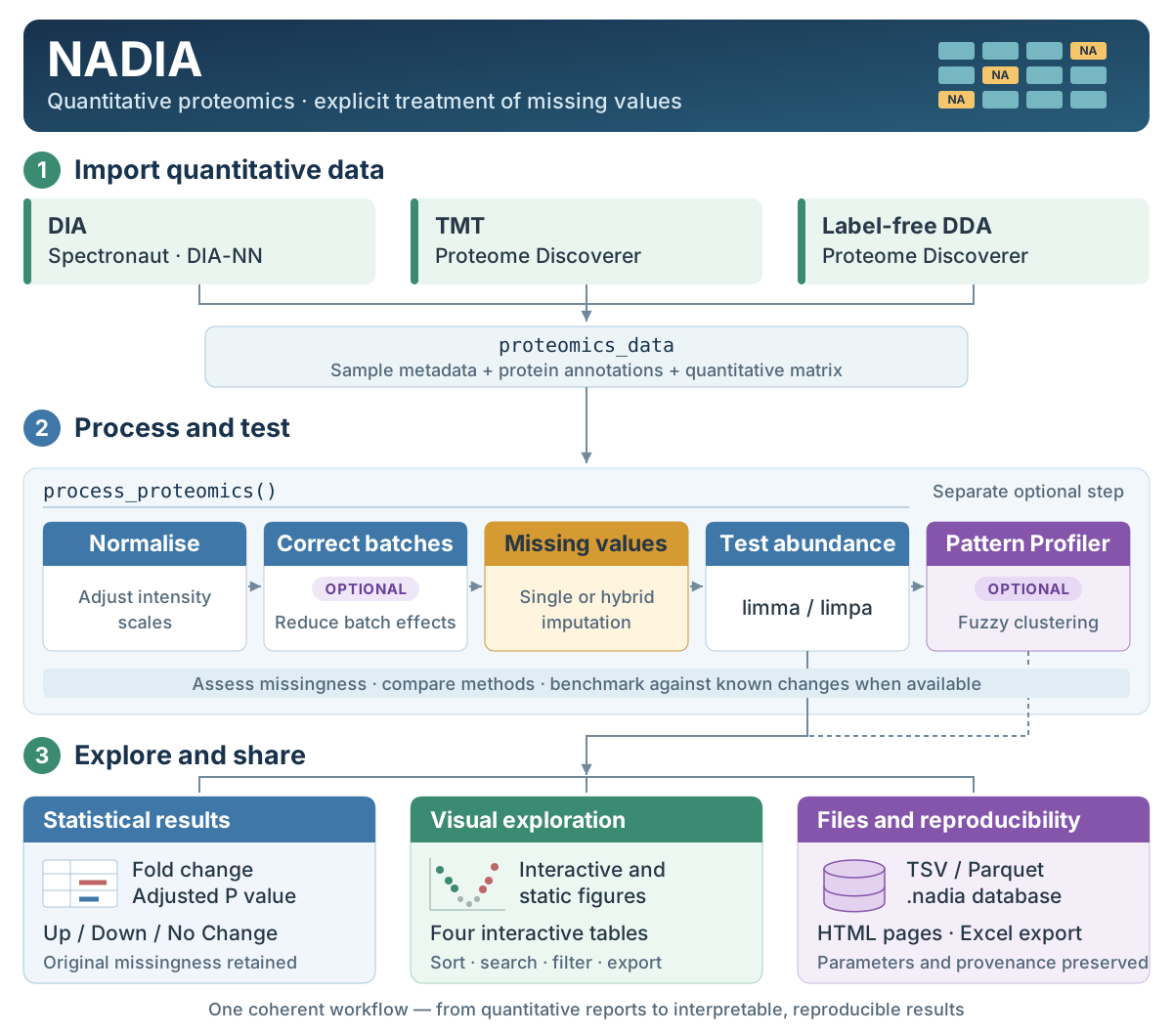
NADIA at a glance: a common workflow from quantification reports to interpretable, reproducible results, with explicit attention to missing values.

The name NADIA is derived from Missing Value-Aware Differential Abundance Analysis of DIA Proteomics Data, which summarises the package’s main purpose: analysing differential protein abundance while explicitly accounting for missing values. The name also brings together NA, the notation used by R for missing values, and DIA, data-independent acquisition, the proteomics context in which the package was initially developed. Although NADIA also processes TMT and label-free DDA data, the assessment and treatment of missing values remain central to its workflow because they are particularly frequent and consequential in DIA experiments.

Why missing values matter

DIA proteomics datasets often contain a substantial proportion of missing values. These values do not always represent random measurement failures. A protein may fall below the limit of detection in one condition and be quantifiable in another, producing precisely the pattern that a differential abundance analysis sets out to identify.

For this reason, removing every protein that contains missing values may discard relevant biological signal. Equally, imputing them without considering the likely mechanism of missingness may attenuate real differences or introduce artificial ones.

This relationship can be observed in the example dataset included with NADIA. The table below groups differential-abundance results by the percentage of missing values within each comparison and their classification as Up, Down or No Change:

Missing values	Up	Down	No Change
0%	795	209	3761
1–25%	90	57	239
26–50%	70	619	54
> 50%	30	52	15

Note: counts refer to protein group–comparison pairs, not unique proteins. The same protein group may appear in more than one comparison.

Most results with no missing values are classified as No Change. Among results with 26–50% missing values, Down classifications are much more frequent than Up classifications: 619 compared with 70.

This pattern is consistent with abundance-dependent missingness, although it does not establish the cause of each missing value. When a protein falls below the detection limit in one condition, missing values can concentrate in the lower-abundance group. NADIA is designed to retain, examine and explicitly handle this information, rather than to remove it or impute it without assessing the consequences.

What NADIA covers

NADIA covers five main areas, from importing quantification reports to exploring and exporting reproducible results:

Import and preprocessing — Reads quantification reports from Spectronaut and DIA-NN, as well as TMT and label-free (DDA) experiments processed with Proteome Discoverer. Every format is converted into a common proteomics_data object, so that the rest of the workflow is independent of the source software.
Processing and differential abundance — Offers 13 normalisation methods, batch-effect assessment and correction, and 20 individual imputation methods. Hybrid imputation strategies handle values assumed to be missing at random (MAR) and missing not at random (MNAR) separately. Differential abundance is analysed with limma or limpa.
Method assessment and selection — Compares normalisation and imputation methods using data-derived metrics. Where a known reference is available, such as a spike-in experiment, NADIA evaluates sensitivity, specificity and the recovery of the expected changes, and ranks normalisation and imputation combinations using the OpDEA approach.
Results exploration and visualisation — Produces interactive figures with Highcharts, including volcano plots, boxplots, principal component analysis (PCA) plots and protein cluster profiles. It also produces static figures with ggplot2 and ComplexHeatmap, and identifies proteins with similar profiles through fuzzy clustering.
Tables and export — Presents the results in interactive tables and exports the processed matrices, the differential abundance results and the data used by the visualisations in formats suited to archiving or further analysis. The analysis can also be saved as a single .nadia file: a DuckDB database that avoids unnecessary duplication and preserves results, parameters and provenance.

Method choice is not cosmetic

Normalisation and imputation are not merely technical steps. They can substantially change the outcome of a differential abundance analysis.

The table below compares four normalisation and imputation combinations applied to the same dataset, using the same statistical model and the same significance and fold-change thresholds:

Pipeline	Up	Down	No Change
`cycloess` + `combo`	985	937	4069
`cycloess` + `knn`	872	179	4940
`quantile` + `combo`	902	2825	2264
`log2` + `min`	761	778	4452

Note: counts refer to protein group–comparison pairs; the same protein group may appear in more than one comparison.

The number of results classified as Down ranges from 179 to 2,825, a roughly sixteen-fold difference. The total number classified as differentially abundant also changes considerably: from around 1,050 with cycloess + knn to more than 3,700 with quantile + combo.

This variability does not by itself indicate which pipeline is correct. It shows that the choice of normalisation and imputation method should be assessed on the data, rather than adopted by convention alone. It also shows why a reproducible analysis must state which methods and parameters produced the final table: without that information, two analyses of the same quantification matrix can lead to very different conclusions.

vignette("choosing-methods") shows how to compare the alternatives when no known reference is available. When the experiment contains a spike-in with expected changes, vignette("benchmarking") evaluates them against that reference.

Installation

NADIA requires R 4.6 or later. While the package is under development and not yet available on Bioconductor, it can be installed from its GitHub repository:

# install.packages("remotes")
remotes::install_github("sciordia/NADIA", build_vignettes = TRUE)
library(NADIA)

The mandatory dependencies declared in the Imports: field of DESCRIPTION are installed automatically. The dependencies declared in Suggests: are only needed for particular optional functions or methods. mice, for instance, is required when that imputation method is selected, pROC computes the AUC and pAUC benchmarking metrics, and Mfuzz is used by the Pattern Profiler.

When an optional dependency is missing, NADIA names the required package and explains how to install it. All the package dependencies can be checked or installed through the helper functions included in the repository:

source("install_dependencies.R")         # from a clone of the repository
install_nadia_deps(dry_run = TRUE)       # only report what is missing
install_nadia_deps(optional = FALSE)     # only the essentials

Once NADIA is available on Bioconductor, the recommended installation will be:

if (!requireNamespace("BiocManager", quietly = TRUE))
    install.packages("BiocManager")
BiocManager::install("NADIA")

A note on Highcharts licensing

NADIA uses the R package highcharter, distributed under the MIT licence, to generate some of its interactive visualisations. highcharter acts as an interface to the Highcharts JavaScript library, which is distributed under its own licensing terms.

NADIA’s licence neither grants nor implies a licence to use Highcharts. Depending on the context in which the visualisations are used — personal, educational, academic, institutional, governmental or commercial — a specific Highcharts licence may be required. Users should consult the current Highsoft terms and ensure that their use complies with the applicable licence.

NADIA’s statistical analysis does not depend on producing interactive figures. The static visualisations produced with ggplot2 and ComplexHeatmap can be used instead, and the complete workflow can be run without generating a single Highcharts figure.

A first analysis

NADIA includes nadia_dia, a preprocessed DIA dataset with three conditions, four replicates per condition and 2,000 protein groups. Approximately 8% of its intensity measurements are missing.

The example below normalises the data with cycloess, applies the hybrid combo imputation strategy and runs the differential abundance analysis with limma:

library(NADIA)

# Preprocessed example dataset
data(nadia_dia)

res <- process_proteomics(
    nadia_dia,
    norm_method = "cycloess",
    imp_method  = "combo",
    mar_method  = "Impseqrob",   # Default MAR method for combo
    mnar_method = "min",         # Default MNAR method for combo
    de_method   = "limma"
)

head(res$DEPs_results)

Here, combo applies a hybrid imputation strategy: Impseqrob handles values classified as MAR, and min handles those classified as MNAR. These are the defaults when mar_method and mnar_method are omitted; either method can be changed through its corresponding argument. The imputed matrix is stored in the Impseqrob_min assay.

process_proteomics() coordinates the main stages of the analysis and returns a list containing the processed object, the differential abundance results and the tables used by the visualisation modules. res$DEPs_results holds one row per protein group and comparison analysed.

The function writes no files unless a directory is given through export_dir.

Alongside logFC, P.Value, adj.P.Val and the classification in Change, the results table retains information about the values that were missing before imputation:

MissGlobal — the percentage of missing values for that protein group across all samples, including conditions outside the current comparison.
MissComp — the percentage of missing values across samples in the two conditions being compared. It can differ from MissGlobal when the experiment includes more than two conditions.
MissCND1 and MissCND2 — the percentage of missing values in each of the two conditions separately.

These columns help distinguish estimates supported by observed intensities from those that depend heavily on imputation; they do not establish biological significance on their own. A protein quantified in only one condition may be absent from the other or below its detection limit. Its logFC and statistical significance should therefore be interpreted in the context of the imputation method used.

To start from a Spectronaut quantification report instead, import it with preprocess_spectronaut(). The resulting prep object can be passed directly to the same processing function:

prep <- preprocess_spectronaut(
    system.file("extdata", "nadia_dia_report.tsv.gz", package = "NADIA"),
    condition_order = c("A", "B", "D")
)

res_from_report <- process_proteomics(
    prep,
    norm_method = "cycloess",
    imp_method  = "combo",
    de_method   = "limma"
)

Documentation and suggested reading

NADIA includes nine vignettes documenting the complete workflow and its main modules. To get started, read vignette("NADIA"), which walks through an analysis from the quantification data to the differential abundance results and their visualisations.

Use the following guide to find the vignette that addresses your question:

Vignette	Question it answers
`NADIA`	How do I run a complete analysis with NADIA?
`input-formats`	How do I import DIA, TMT or label-free (DDA) data?
`missing-values`	What do the missing values mean and how should I impute them?
`choosing-methods`	How do I compare normalisation and imputation methods without a known reference?
`benchmarking`	How do I evaluate pipelines when I have a spike-in experiment with expected changes?
`batch-correction`	How do I detect batch effects, correct them and assess the correction?
`pattern-profiler`	How do I identify proteins with similar profiles across conditions?
`visualization`	How do I customise the interactive and static figures?
`results-and-export`	How do I export, archive and share the analysis results?

Every vignette contains executable code and generates its results from the datasets shipped with the package, so the examples can be reproduced and adapted to other experiments.

The installed vignettes can be browsed with browseVignettes("NADIA").

Running NADIA from a coding assistant

NADIA ships an agent skill: the same pipeline written for a coding assistant rather than for a reader. It documents which function to call at each stage, how to choose between the normalisation and imputation methods, what to check afterwards, and the mistakes the package’s defaults invite. It is plain Markdown, so any assistant can read it, and it follows the layout Claude expects for a skill.

nadia_skill_path()          # where the skill is installed

To use it with Claude Code, copy that directory into the skills folder of your project or of your user account:

cp -R "$(Rscript -e 'cat(NADIA::nadia_skill_path())')" ~/.claude/skills/nadia

The source lives in inst/skill/ in this repository.

Package architecture

NADIA has a modular architecture. The functions below can be used independently in a custom workflow or through the main analysis pipeline.

Import and preprocessing

The preprocessing functions convert the different input formats into a common structure:

preprocess_spectronaut() handles Spectronaut quantification reports in long format.
preprocess_diann() handles wide-format DIA-NN protein-group matrices (report.pg_matrix.tsv).
preprocess_tmt() handles TMT reports exported by Proteome Discoverer.
preprocess_lfq() handles label-free reports exported by Proteome Discoverer.

For the three wide formats, NADIA reads the experimental design from column names following the Abundance: <condition>_<replicate> convention. Alternatively, a two-column sample annotation file can be supplied through annot_path.

All four return a proteomics_data object with the same basic structure: sample metadata, protein annotation and the quantification matrix. The later stages therefore apply in the same way regardless of the source software or quantification design.

Main processing

process_proteomics() coordinates the central stages of the analysis:

normalisation
optional batch-effect correction
imputation of missing values
differential abundance analysis

Pattern Profiler is a separate optional step. It is run afterwards with pattern_profiler_analysis(), which identifies proteins with similar abundance profiles from the processed object and the differential abundance results.

From normalisation onwards, NADIA stores the data in a SummarizedExperiment. Assays contain quantitative matrices with protein groups in rows and samples in columns; rowData and colData store the corresponding protein annotations and sample metadata. These components remain aligned when the object is subsetted.

Separate assays preserve the input, log-transformed, normalised and imputed matrices. The function also returns the differential-abundance results and the tables used by the visualisation modules.

The main stages can be run individually through normalize_proteomics(), batch_correct_proteomics(), impute_proteomics() and de_analysis_proteomics().

Assessment and benchmarking

The assessment modules are separate from the main processing:

normalization_metrics() compares normalisation methods using observable properties of the data.
imputation_metrics() evaluates imputation methods by simulating missing values.
benchmarking_proteomics() compares one pipeline against the expected changes of a spike-in experiment.
benchmarking_multiple() ranks multiple normalisation and imputation combinations.

Visualisation and presentation of results

The visualisation functions mainly accept tables and data frames, so they can be used both with the results of process_proteomics() and with results produced elsewhere.

NADIA provides interactive volcano, boxplot, PCA and cluster-profile figures, static figures through ggplot2 and ComplexHeatmap, and interactive tables built on reactable.

Example data and provenance

The example data shipped with NADIA come from quantitative proteomics experiments conducted at the Proteomics Facility of the Centro Nacional de Biotecnología (CNB-CSIC).

The package includes:

nadia_dia, a preprocessed proteomics_data object that allows the main workflow to be run directly;
trimmed Spectronaut, DIA-NN, TMT and label-free (DDA) quantification reports, stored in inst/extdata/, which demonstrate the import and preprocessing functions for each format;
the additional information needed for the spike-in benchmarking examples.

All four reports include conditions A, B and D. The Spectronaut, DIA-NN and LFQ examples contain four replicates per condition. Spectronaut and DIA-NN process the same twelve DIA injections, allowing the effects of data processing on missingness to be compared before imputation.

The TMT report comes from a separate experiment with the same three-proteome spike-in design. It contains eight replicates per condition across two TMT mixes: replicates 1–4 belong to the first mix, and replicates 5–8 to the second. Four internal-standard channels link the mixes, providing a real batch structure for the batch-correction examples.

The distributed reports contain a random subset of 2,000 protein groups drawn from the full experiments. Random selection, rather than selecting only the most complete proteins, helps preserve realistic missing-value patterns.

The full experimental datasets are unpublished and are not included in the package or repository. The script inst/scripts/make_extdata.R documents how the example reports and the nadia_dia object were prepared from the original data.

These data are provided solely to demonstrate, test and reproduce the behaviour of the package. They should not be treated as reference datasets from which to draw biological conclusions about the original experiments.

License

NADIA is free and open-source software distributed under the terms of the GNU General Public License, version 3 or any later version. The code may be used, modified and redistributed in accordance with the conditions of that licence. See the LICENSE file and the License: field of DESCRIPTION for further details.