Results and export: sharing and preserving an analysis

Introduction

A proteomics analysis should finish with outputs that other people can inspect and that the analyst can reproduce later. NADIA supports several complementary routes: selected tables can be exported as TSV or Parquet files, a complete run can be archived in one .nadia file, and interactive tables or figures can be shared as HTML.

This vignette explains when to use each route, how to create the corresponding files, and how to verify what has been saved. The examples use the bundled DIA dataset so that every output can be reproduced without external files.

Prepare an example analysis

This section creates one NADIA result that will be reused throughout the vignette. Keeping a single analysis object also makes it easier to compare the different export formats.

Install and load NADIA

Install NADIA through Bioconductor if it is not already available, and then load the package and example data.

if (!requireNamespace("BiocManager", quietly = TRUE)) {
  install.packages("BiocManager")
}
BiocManager::install("NADIA")

library(NADIA)
data(nadia_dia)

Run the processing workflow

process_proteomics() returns all analysis components in memory. Because export_dir is not supplied here, this call does not create any files.

res <- process_proteomics(
  nadia_dia,
  verbose = FALSE
)

The returned object contains the processed experiment, differential-abundance results, plotting tables, comparison names, and the parameters used in the run. The following code summarises the size and purpose of the main components used throughout this vignette.

Show the code used to summarise the returned components

component_summary <- data.frame(
  Component = c(
    "se_proc",
    "DEPs_results",
    "BoxPlot_Input",
    "PCA_Input",
    "comparisons",
    "parameters"
  ),
  Rows = c(
    nrow(res$se_proc),
    nrow(res$DEPs_results),
    nrow(res$BoxPlot_Input),
    nrow(res$PCA_Input),
    length(res$comparisons),
    length(res$parameters)
  ),
  Columns = c(
    ncol(res$se_proc),
    ncol(res$DEPs_results),
    ncol(res$BoxPlot_Input),
    ncol(res$PCA_Input),
    "\u2014",
    "\u2014"
  ),
  Purpose = c(
    "Processed assays and sample metadata",
    "Differential-abundance statistics",
    "Long-format intensities for boxplots",
    "Long-format intensities and significance flags for PCA",
    "Available pairwise comparisons",
    "Analysis settings and recorded function call"
  ),
  check.names = FALSE
)

knitr::kable(
  component_summary,
  caption = "Main components returned by process_proteomics().",
  align = c("l", "r", "r", "l")
)

Main components returned by process_proteomics().
Component	Rows	Columns	Purpose
se_proc	1997	12	Processed assays and sample metadata
DEPs_results	5991	12	Differential-abundance statistics
BoxPlot_Input	47928	6	Long-format intensities for boxplots
PCA_Input	23964	9	Long-format intensities and significance flags for PCA
comparisons	3	—	Available pairwise comparisons
parameters	38	—	Analysis settings and recorded function call

The values are calculated directly with nrow() and ncol(), but the row count reflects the structure of each object rather than the number of unique proteins. DEPs_results contains 1,997 proteins across three comparisons (5,991 rows), BoxPlot_Input contains the same proteins across 12 samples and two assays (47,928 rows), and PCA_Input contains one row per protein and sample (23,964 rows). In the three data frames, Columns counts the available variables; in se_proc, its 1,997 rows and 12 columns correspond directly to proteins and samples, respectively. The final two components are not tabular: comparisons contains three contrast names and parameters contains 38 recorded analysis entries, so Columns is not applicable to them.

Choose an output for the task

The most appropriate output depends on who will use it and whether they need selected results or the complete analysis. The following diagram compares the four main options used in this vignette.

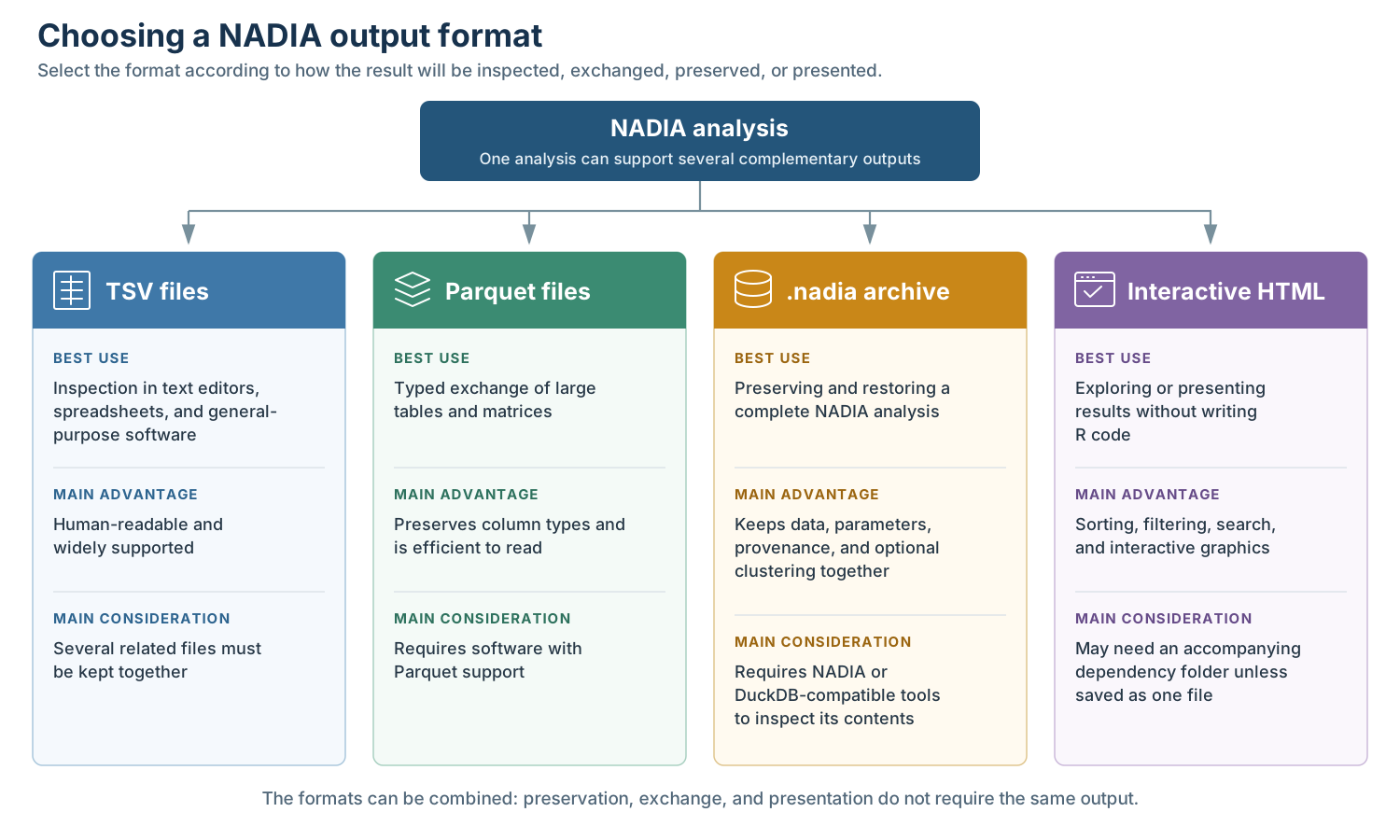
A NADIA analysis branches into TSV files, Parquet files, a .nadia archive, and interactive HTML. Each output is described by its best use, main advantage, and main consideration.

Four complementary formats for exporting, preserving, or presenting NADIA results.

Click the figure to enlarge it; press Esc or click outside the image to close it.

The four formats address different priorities. TSV files favour immediate, human-readable inspection, whereas Parquet preserves column types for efficient programmatic exchange. A .nadia archive is the most complete option for restoring the analysis and its provenance, while interactive HTML is designed for exploration and presentation without R code. These outputs are complementary: a practical workflow can retain the .nadia archive as the master record, export TSV or Parquet tables for downstream use, and share HTML with collaborators for interactive review.

Export tabular results

Having introduced the file formats supported by NADIA, we now examine them in turn, beginning with TSV and Parquet. Both can store the same result tables; the choice affects only how they are stored and read. This section first compares the two formats and then shows how to export either one, or both, directly from process_proteomics().

Choose between TSV and Parquet

TSV and Parquet store the same tabular information in different ways. TSV is tab-separated plain text that can be opened directly in a text editor or spreadsheet, making it convenient for manual inspection and exchange. However, column types must be inferred when it is read, and large files can require considerable disk space.

Parquet is a compressed, binary columnar format widely used in data analytics. Storing values by column allows software to read only the data it needs, making access faster and files smaller. Because Parquet is not human-readable, it requires compatible software: in R, arrow::read_parquet() can load it into memory, while DuckDB can query it directly.

The following table compares the main characteristics of the TSV and Parquet formats.

Show the code used to compare TSV and Parquet

format_guide <- data.frame(
  Property = c(
    "File structure",
    "Readable as plain text",
    "Direct manual inspection",
    "Column types",
    "Storage requirement",
    "Repeated programmatic access",
    "Typical use"
  ),
  TSV = c(
    "Tab-delimited text",
    "Yes",
    "Text editor or spreadsheet",
    "Inferred when imported",
    "Larger for substantial tables",
    "Requires parsing the text",
    "Review, exchange, and small analyses"
  ),
  Parquet = c(
    "Compressed columnar binary",
    "No",
    "Requires Parquet-aware software",
    "Stored in the file schema",
    "Usually smaller",
    "Fast, including selected-column reads",
    "Data analytics and automated workflows"
  ),
  check.names = FALSE
)

knitr::kable(
  format_guide,
  caption = "Practical differences between TSV and Parquet exports.",
  align = c("l", "l", "l")
)

Practical differences between TSV and Parquet exports.
Property	TSV	Parquet
File structure	Tab-delimited text	Compressed columnar binary
Readable as plain text	Yes	No
Direct manual inspection	Text editor or spreadsheet	Requires Parquet-aware software
Column types	Inferred when imported	Stored in the file schema
Storage requirement	Larger for substantial tables	Usually smaller
Repeated programmatic access	Requires parsing the text	Fast, including selected-column reads
Typical use	Review, exchange, and small analyses	Data analytics and automated workflows

In summary, TSV is best for simple inspection and exchange, whereas Parquet is better suited to large datasets and repeated computational analysis because it is smaller, faster to read, and preserves column types. Use both when manual readability and efficient processing are equally important.

Create a set of TSV and/or Parquet files

process_proteomics() can write processed matrices and plotting inputs while it runs. Export is activated only when export_dir is supplied; with its default value of NULL, all results remain in memory and no directory or file is created. The value of export_format then selects TSV, Parquet, or a matched copy in both formats.

Main export arguments of process_proteomics()

export_dir gives the destination directory. Its default value, NULL, disables every file export.
export_format accepts "tsv", "parquet", or "both". The last option writes the same selected tables in both representations. Parquet export through process_proteomics() requires the arrow package.
export_normalized and export_imputed control the processed intensity matrices.
export_volcano, export_boxplot, and export_pca control the tables used by the corresponding visualisation functions.

The following alternatives differ only in export_dir and export_format. Run the one that matches the intended downstream use; repeating the full analysis three times is not necessary.

# Export one TSV file for every enabled output.
process_proteomics(
  nadia_dia,
  export_dir = "results/tsv",
  export_format = "tsv",
  verbose = FALSE
)

# Export the same outputs only as compressed Parquet files.
process_proteomics(
  nadia_dia,
  export_dir = "results/parquet",
  export_format = "parquet",
  verbose = FALSE
)

# Export matched TSV and Parquet copies of every enabled output.
process_proteomics(
  nadia_dia,
  export_dir = "results/tsv_and_parquet",
  export_format = "both",
  verbose = FALSE
)

With the default export switches, NADIA writes five datasets: the normalised intensity matrix (export_normalized), the final imputed matrix (export_imputed), the differential-abundance results used by the volcano plots (export_volcano), the long-format intensities used by the boxplots (export_boxplot), and the imputed intensities with significance annotations used by PCA and heatmaps (export_pca). The matrix files contain one protein per row and one sample per intensity column, whereas the plotting inputs use long or results-oriented layouts suited to their downstream functions. File names include the normalisation and imputation methods so that outputs from different runs can be distinguished.

The next call writes all five default outputs as TSV files to a temporary directory and displays the types of files generated. In a real analysis, replace export_dir with a permanent project directory.

Show the code used to create the export manifest

export_dir <- file.path(tempdir(), "nadia_vignette_tables")
unlink(export_dir, recursive = TRUE)

invisible(process_proteomics(
  nadia_dia,
  export_dir = export_dir,
  export_format = "tsv",
  verbose = FALSE
))

exported_files <- list.files(export_dir, full.names = TRUE)

file_contents <- ifelse(
  grepl("matrix_log2.*Imp", basename(exported_files)),
  "Imputed intensity matrix",
  ifelse(
    grepl("matrix_log2", basename(exported_files)),
    "Normalised intensity matrix",
    ifelse(
      grepl("VolcanoPlot", basename(exported_files)),
      "Differential-abundance results",
      ifelse(
        grepl("BoxPlot", basename(exported_files)),
        "Long-format boxplot input",
        "Long-format PCA input"
      )
    )
  )
)

export_manifest <- data.frame(
  File = basename(exported_files),
  Contents = file_contents,
  Size = sprintf("%.1f KB", file.info(exported_files)$size / 1024),
  check.names = FALSE
)

knitr::kable(
  export_manifest,
  caption = "Files created by the default TSV export.",
  align = c("l", "l", "r")
)

Files created by the default TSV export.
File	Contents	Size
BoxPlot_Input_cycloess_Impseqrob_min.tsv	Long-format boxplot input	1999.3 KB
matrix_log2_cycloess_Impseqrob_min.tsv	Imputed intensity matrix	450.1 KB
matrix_log2_cycloess.tsv	Normalised intensity matrix	423.1 KB
PCA_Input_cycloess_Impseqrob_min.tsv	Long-format PCA input	2317.0 KB
VolcanoPlot_Input_cycloess_Impseqrob_min.tsv	Differential-abundance results	635.8 KB

The filenames record the normalisation and imputation methods, reducing the risk of mixing tables from different runs. The plotting inputs are intentionally long: each row represents an observation required by its corresponding plot, whereas the two matrix files keep one protein per row.

Exports can also be assembled à la carte with the five switches shown above. Each export_* argument is TRUE by default; set it to FALSE to omit that dataset. The value of export_format is applied to every dataset that remains enabled. The following example requests matching TSV and Parquet copies of only the final imputed matrix and the differential-abundance results; the normalised matrix and the boxplot and PCA inputs are omitted.

process_proteomics(
  nadia_dia,
  export_dir = "results/selected_tables",
  export_format = "both",
  export_normalized = FALSE,
  export_imputed = TRUE,
  export_volcano = TRUE,
  export_boxplot = FALSE,
  export_pca = FALSE,
  verbose = FALSE
)

Archive a complete analysis

Separate tables are useful for exchange, but they do not by themselves retain the complete relationship between preprocessing, processing, parameters, and provenance. write_nadia() stores these elements in a single DuckDB database using the .nadia extension.

Write and read a .nadia file

The required input is the preprocessing object. The processing result and a Pattern Profiler result can be included when available.

Main arguments of write_nadia()

file is the path of the archive to create.
preprocessing is the proteomics_data object returned by a NADIA preprocessing function.
result is the optional output from process_proteomics().
pattern_profiler optionally adds the output from pattern_profiler_analysis().
overwrite = TRUE explicitly replaces an existing archive.

The following example creates a .nadia archive from the bundled dataset and summarises selected file characteristics and metadata in the table below.

Show the code used to create and summarise the .nadia archive

nadia_file <- file.path(tempdir(), "nadia_vignette_analysis.nadia")
unlink(c(nadia_file, paste0(nadia_file, ".wal")))

write_nadia(
  nadia_file,
  preprocessing = nadia_dia,
  result        = res,
  verbose       = FALSE
)

db <- read_nadia(nadia_file)

archive_summary <- data.frame(
  Property = c(
    "Archive size",
    "Samples",
    "Proteins",
    "Normalised assay",
    "Imputed assay",
    "Pattern Profiler stored"
  ),
  Value = c(
    sprintf("%.1f MB", file.size(nadia_file) / 1024^2),
    db$meta[["n_samples"]],
    db$meta[["n_proteins"]],
    db$meta[["norm_assay"]],
    db$meta[["imputed_assay"]],
    db$meta[["has_pattern_profiler"]]
  ),
  check.names = FALSE
)

knitr::kable(
  archive_summary,
  caption = "Summary of the example .nadia archive.",
  align = c("l", "l")
)

Summary of the example .nadia archive.
Property	Value
Archive size	4.0 MB
Samples	12
Proteins	2000
Normalised assay	cycloess
Imputed assay	Impseqrob_min
Pattern Profiler stored	FALSE

This initial archive contains the complete preprocessing and processing run; Pattern Profiler stored is therefore FALSE. Section 5.5 adds the optional clustering result to the same archive. If clustering has already been completed, it can instead be supplied directly to write_nadia() through pattern_profiler.

Restore and verify the result

NADIA provides three functions for restoring a .nadia archive and converting its contents back into the tables and objects generated during the original analysis:

read_nadia() opens the archive and exposes its metadata, canonical tables, and stored views through a nadia_db object.
nadia_result() reconstructs the proteomics_result returned by process_proteomics(), ready for NADIA plotting and reporting functions.
nadia_preprocessing() restores the original proteomics_data object so that the processing workflow can be run again.

The following code verifies that the tables and objects restored from the .nadia archive are identical to those generated during the original analysis.

Show the code used to verify the restored results

restored <- nadia_result(db)

roundtrip_check <- data.frame(
  Component = c(
    "Differential-abundance results",
    "PCA input",
    "Final imputed assay"
  ),
  Identical = c(
    identical(restored$DEPs_results, res$DEPs_results),
    identical(restored$PCA_Input, res$PCA_Input),
    identical(
      SummarizedExperiment::assay(restored$se_proc, "Impseqrob_min"),
      SummarizedExperiment::assay(res$se_proc, "Impseqrob_min")
    )
  ),
  check.names = FALSE
)

knitr::kable(
  roundtrip_check,
  caption = "Round-trip verification after restoring the archive.",
  align = c("l", "c")
)

Round-trip verification after restoring the archive.
Component	Identical
Differential-abundance results	TRUE
PCA input	TRUE
Final imputed assay	TRUE

All three checks return TRUE, confirming that the tables, their column types, and the final assay are reproduced exactly in this example.

Inspect stored tables and provenance

The .nadia file avoids unnecessary duplication. Values that can be reconstructed exactly, such as the log2 assay and PCA_Input, are exposed through SQL views rather than stored as additional copies. For imputation methods that leave observed values unchanged, only the replaced cells and their MAR or MNAR branch need to be stored.

The following table lists the SQL views from which NADIA can reconstruct the original content of the analysis.

Show the code used to inspect the SQL views

archive_views <- subset(nadia_tables(nadia_file), type == "view")

view_description <- c(
  v_boxplot_input = "Boxplot input",
  v_deps_results = "Differential-abundance results",
  v_matrix_imputed = "Final imputed matrix",
  v_matrix_norm = "Normalised matrix",
  v_metadata = "Sample metadata",
  v_pca_input = "PCA input",
  v_protein_id = "Protein identification table",
  v_protein_quant = "Protein quantification table"
)

archive_views$Contents <- unname(view_description[archive_views$name])

knitr::kable(
  archive_views[, c("name", "rows", "Contents")],
  col.names = c("View", "Rows", "Reconstructed contents"),
  caption = "Canonical views available in the example archive.",
  align = c("l", "r", "l"),
  row.names = FALSE
)

Canonical views available in the example archive.
View	Rows	Reconstructed contents
v_boxplot_input	47928	Boxplot input
v_deps_results	5991	Differential-abundance results
v_matrix_imputed	1997	Final imputed matrix
v_matrix_norm	1997	Normalised matrix
v_metadata	12	Sample metadata
v_pca_input	23964	PCA input
v_protein_id	2000	Protein identification table
v_protein_quant	2000	Protein quantification table

The views provide the same analysis tables that users normally access in R. The archive also records package versions, function calls, source-file information, and analysis parameters.

Show the code used to inspect the stored parameters

provenance_parameters <- subset(
  db$parameters,
  name %in% c(
    "norm_method", "imp_method", "mar_method", "mnar_method",
    "de_method", "alpha", "logFC_threshold"
  )
)

knitr::kable(
  provenance_parameters[, c("step", "name", "value")],
  col.names = c("Stage", "Parameter", "Recorded value"),
  caption = "Selected parameters stored in the .nadia archive.",
  align = c("l", "l", "l"),
  row.names = FALSE
)

Selected parameters stored in the .nadia archive.
Stage	Parameter	Recorded value
process	norm_method	cycloess
process	imp_method	combo
process	mar_method	Impseqrob
process	mnar_method	min
process	logFC_threshold	0
process	alpha	0.05
process	de_method	limma

These values identify the main analysis choices rather than merely describing the exported table.

Query or extract the archive

Because a .nadia file is itself a DuckDB database, nadia_connect() can open a DBI connection for targeted SQL queries. DuckDB executes these queries directly, without reconstructing the complete analysis in R. The following example counts proteins in the three differential-abundance categories for each comparison.

Show the code used to query protein counts with SQL

con <- nadia_connect(nadia_file)

sql_summary <- DBI::dbGetQuery(
  con,
  paste(
    'SELECT "Comparison", "Change", COUNT(*) AS "Proteins"',
    'FROM v_deps_results',
    'GROUP BY "Comparison", "Change"',
    'ORDER BY "Comparison", "Change"'
  )
)

DBI::dbDisconnect(con, shutdown = TRUE)

knitr::kable(
  sql_summary,
  caption = "Protein counts queried directly from the .nadia archive.",
  align = c("l", "l", "r")
)

Protein counts queried directly from the .nadia archive.
Comparison	Change	Proteins
B-A	Down	172
B-A	No Change	1500
B-A	Up	325
D-A	Down	383
D-A	No Change	1240
D-A	Up	374
D-B	Down	382
D-B	No Change	1329
D-B	Up	286

These SQL queries reproduce the counts of statistically significant proteins in each comparison using the stored Change classifications, which reflect the adjusted-p-value and fold-change criteria defined in the original analysis.

To work with software that cannot read .nadia files, NADIA provides nadia_export_parquet() to export each canonical view directly as a Parquet file. This export is performed by DuckDB directly and therefore does not require arrow. The following table lists all Parquet tables extracted from the example .nadia file.

Show the code used to export the canonical views to Parquet

parquet_dir <- file.path(tempdir(), "nadia_vignette_parquet")
unlink(parquet_dir, recursive = TRUE)
invisible(nadia_export_parquet(db, parquet_dir, verbose = FALSE))

parquet_manifest <- data.frame(
  File = list.files(parquet_dir),
  check.names = FALSE
)

knitr::kable(
  parquet_manifest,
  caption = "Parquet tables extracted from the .nadia archive.",
  align = "l"
)

Parquet tables extracted from the .nadia archive.
File
nadia_calls.parquet
nadia_meta.parquet
nadia_packages.parquet
nadia_source_files.parquet
parameters.parquet
v_boxplot_input.parquet
v_deps_results.parquet
v_matrix_imputed.parquet
v_matrix_norm.parquet
v_metadata.parquet
v_pca_input.parquet
v_protein_id.parquet
v_protein_quant.parquet

Working location. Do not keep an open .nadia database inside a folder that is being synchronised by iCloud Drive, Dropbox, or OneDrive. Write and use the archive in a local directory, close it, and then copy the completed file to the synchronised location.

Combine differential abundance with clustering

An existing .nadia file can optionally be extended with the results of a Pattern Profiler analysis. The following code generates the clustering result pp from the processed data and adds it to the file with nadia_add_pattern_profiler().

Show the code used to run and store Pattern Profiler

# Generate expression-pattern clusters.
pp <- pattern_profiler_analysis(
  res$se_proc,
  res$DEPs_results,
  assay_name = "Impseqrob_min",
  seed       = 123,
  verbose    = FALSE
)

# Add the clustering results to the existing .nadia file.
nadia_add_pattern_profiler(
  nadia_file,
  pattern_profiler = pp,
  verbose = FALSE
)

For downstream functional or enrichment analyses, NADIA can retrieve differential-abundance statistics together with expression-pattern assignments from the .nadia file. deps_with_clusters() combines these results in memory, whereas nadia_deps_with_clusters() reads the equivalent table from a .nadia archive. Both return the columns of DEPs_results followed by Cluster, Membership, and ClusterRank; rank 1 identifies the dominant cluster of a protein.

Main arguments of deps_with_clusters()

DEPs_results supplies the differential-abundance statistics, and pattern_profiler supplies the clustering result (pp).
assignment selects the shape of the result. "primary", the default, keeps the cluster of highest membership and returns one row per protein and comparison. "all" keeps every soft-cluster association retained in long_output; a clustered protein without a retained association still receives its dominant assignment.
min_membership applies an additional threshold to the returned assignments. It can make the selection stricter, but it cannot recover secondary memberships omitted when long_output was created.
comparison restricts the result to selected comparisons.
significant_only keeps only rows classified as Up or Down, using the classification made during the analysis.

The following table shows six clustered proteins, combining their differential-abundance statistics with their dominant cluster and membership.

Show the code used to combine differential-abundance results with dominant clusters

functional_input <- deps_with_clusters(
  res$DEPs_results,
  pp,
  assignment = "primary"
)

knitr::kable(
  head(functional_input[
    !is.na(functional_input$Cluster),
    c("Protein.IDs", "Comparison", "logFC", "adj.P.Val", "Change",
      "Cluster", "Membership")
  ], 6),
  caption = "Differential-abundance results with the dominant cluster of each protein.",
  align = c("l", "l", "r", "r", "l", "r", "r"),
  row.names = FALSE,
  digits = 4
)

Differential-abundance results with the dominant cluster of each protein.
Protein.IDs	Comparison	logFC	adj.P.Val	Change	Cluster	Membership
A0A140T897;P02769	B-A	0.1344	0.0031	Up	2	0.8810
A0A140T897;P02769	D-B	0.2048	0.0001	Up	2	0.8810
A0A140T897;P02769	D-A	0.3392	0.0000	Up	2	0.8810
A6H7B5	D-B	-0.0538	0.0795	No Change	2	0.5814
A6H7B5	D-A	0.0550	0.0644	No Change	2	0.5814
A6H7B5	B-A	0.1088	0.0021	Up	2	0.5814

Each row retains the original statistical results; Cluster identifies the dominant expression pattern, and Membership measures how strongly the protein belongs to it. Because soft clustering can associate a protein with several patterns, the next table compares the row counts for assignment = "primary" and assignment = "all".

Show the code used to compare cluster assignment modes

soft <- deps_with_clusters(res$DEPs_results, pp, assignment = "all")

assignment_summary <- data.frame(
  Table = c(
    "Differential-abundance results",
    "assignment = \"primary\"",
    "assignment = \"all\""
  ),
  Rows = c(nrow(res$DEPs_results), nrow(functional_input), nrow(soft)),
  Proteins_without_cluster = c(
    NA_integer_,
    length(unique(functional_input$Protein.IDs[is.na(functional_input$Cluster)])),
    length(unique(soft$Protein.IDs[is.na(soft$Cluster)]))
  ),
  check.names = FALSE
)

knitr::kable(
  assignment_summary,
  col.names = c("Table", "Rows", "Proteins without a cluster"),
  caption = "Effect of the assignment mode on the number of rows.",
  align = c("l", "r", "r")
)

Effect of the assignment mode on the number of rows.
Table	Rows	Proteins without a cluster
Differential-abundance results	5991	NA
assignment = “primary”	5991	1203
assignment = “all”	6210	1203

"primary" keeps one row per protein and comparison, whereas "all" adds rows for the retained secondary cluster assignments. With these default filters, both modes keep proteins without a cluster (NA), preserving the full set of tested proteins as a potential background for enrichment analysis.

The .nadia file also exposes the combined results through the SQL view v_deps_pattern_profiler, which is included in subsequent Parquet exports. The following query counts proteins by dominant cluster and differential-abundance category for comparison B-A; ClusterRank = 1 ensures that each protein is counted only in its dominant cluster.

Show the code used to query differential-abundance categories by cluster

con <- nadia_connect(nadia_file)

cluster_counts <- DBI::dbGetQuery(
  con,
  paste(
    'SELECT "Cluster", "Change", COUNT(*) AS "Proteins"',
    'FROM v_deps_pattern_profiler',
    'WHERE "ClusterRank" = 1 AND "Cluster" IS NOT NULL',
    'AND "Comparison" = \'B-A\'',
    'GROUP BY "Cluster", "Change"',
    'ORDER BY "Cluster", "Change"'
  )
)

DBI::dbDisconnect(con, shutdown = TRUE)

knitr::kable(
  cluster_counts,
  caption = "Differential-abundance categories per cluster in comparison B-A.",
  align = c("r", "l", "r")
)

The following table summarises the number of proteins in each differential-abundance category within each dominant cluster.

Differential-abundance categories per cluster in comparison B-A.
Cluster	Change	Proteins
1	Down	172
1	No Change	228
1	Up	4
2	No Change	69
2	Up	321

These counts show how differential-abundance categories are distributed across expression patterns. Storing both results in one .nadia file makes them available together through R or SQL for downstream analyses.

Explore results with interactive tables

NADIA provides Reactable-based interactive tables for reviewing analysis results, with sorting, search, filters, and Excel export. Four distinct tables cover sample metadata, annotations for identified proteins, quantification values, and differential-abundance results. Use a *_reactable() function when only the table is required, or a *_widget() function when a complete page with additional controls and Excel export is needed.

The diagram below links each interactive view to its input, row structure, and available functions.

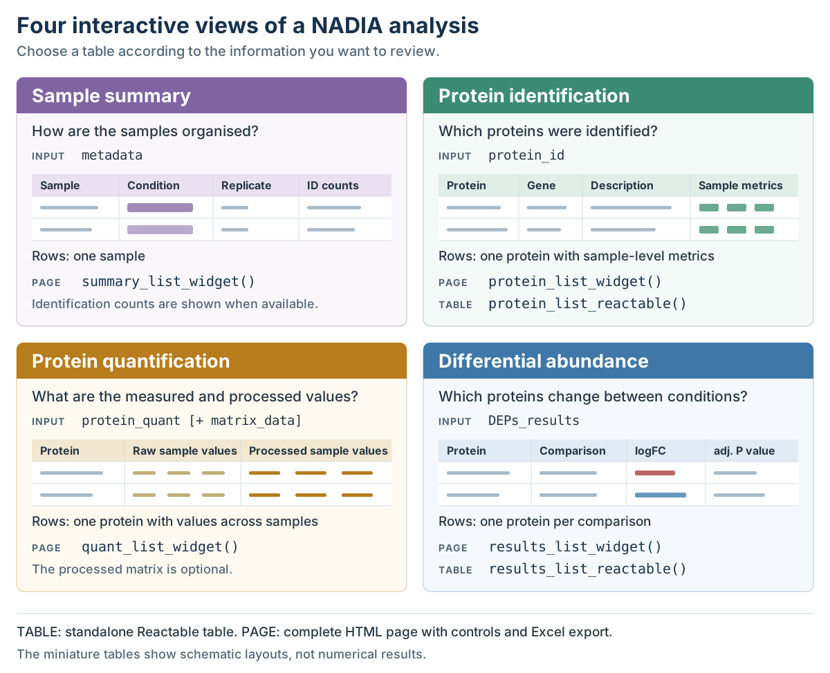
From top left to bottom right: sample summary, protein identification, protein quantification, and differential abundance. Each panel shows a schematic table layout, input objects, row units, and the available NADIA functions.

Four complementary interactive tables for reviewing a NADIA analysis.

Click the figure to enlarge it; press Esc or click outside the image to close it.

The following code creates and displays the four interactive pages in the same order as the diagram, using the example dataset and processing results.

Show the code used to create the four interactive tables

# 1. Sample metadata.
sample_page <- summary_list_widget(nadia_dia$metadata)
sample_page

# 2. Annotations for identified proteins.
protein_page <- protein_list_widget(
  nadia_dia$protein_id,
  metadata = nadia_dia$metadata
)
protein_page

# 3. Quantification values: add the final processed matrix.
imputed_matrix <- SummarizedExperiment::assay(
  res$se_proc,
  "Impseqrob_min"
)
matrix_data <- data.frame(
  ProteinGroups = rownames(imputed_matrix),
  imputed_matrix,
  check.names = FALSE
)

quantification_page <- quant_list_widget(
  nadia_dia$protein_quant,
  matrix_data = matrix_data,
  metadata = nadia_dia$metadata
)
quantification_page

# 4. Differential-abundance results for comparison B-A.
results_page <- results_list_widget(
  res$DEPs_results,
  protein_quant = nadia_dia$protein_quant,
  comparisons = "B-A",
  alpha = 0.05,
  page_size = 15
)
results_page

summary_list_widget() adapts to the available sample metadata, omitting fields absent from the input format.
protein_list_widget() displays protein annotations and sample-level identification metrics.
quant_list_widget() joins the processed matrix to the quantification table through ProteinGroups, which must be present in the matrix.
results_list_widget() provides sorting, search, filters, and Excel export; supplying protein_quant adds protein descriptions and quantified-peptide counts to the statistical results.

Offline Excel export. Each complete *_widget() page includes an Export to Excel button. The workbook is generated in the browser with formatted headers, suitable column widths, and numeric cells stored as numbers.

This export requires two JavaScript libraries: ExcelJS, which creates the formatted .xlsx workbook, and PapaParse, which parses tabular text during browser-side export.

Both libraries and their licence files are shipped with NADIA rather than downloaded from a content-delivery network. The Excel button therefore remains available when the saved page is opened offline, provided its local dependency folder accompanies the HTML file.

Save interactive HTML

An interactive result can be saved either as a complete page plus a dependency folder or, for an individual htmlwidget, as one self-contained HTML file. The choice affects portability and which page controls are retained.

Objects returned by results_list_widget(), protein_list_widget(), quant_list_widget(), and summary_list_widget() are complete HTML pages. htmltools::save_html() saves the page and copies its JavaScript and CSS dependencies into a neighbouring lib directory.

The following example creates and saves an interactive results page for comparison B-A. Replace widget_dir with a permanent project directory to keep the exported page.

Show the code used to save the interactive results page

widget_dir <- file.path(tempdir(), "nadia_vignette_widget")
dir.create(widget_dir, recursive = TRUE, showWarnings = FALSE)

results_page <- results_list_widget(
  res$DEPs_results,
  protein_quant = nadia_dia$protein_quant,
  comparisons = "B-A"
)

htmltools::save_html(
  results_page,
  file.path(widget_dir, "results_B-A.html")
)

The saved page retains the full NADIA toolbar, including filters and Excel export. Keep the HTML file and its lib directory together when moving or sharing the page so that it remains functional offline.

results_list_reactable() and the Highcharts plotting functions return actual htmlwidget objects. They can be embedded into a single HTML file with htmlwidgets::saveWidget(..., selfcontained = TRUE).

The following example creates a results table for comparison B-A and saves it as a single HTML file, using the output directory from the previous example.

Show the code used to save the self-contained HTML file

result_table <- results_list_reactable(
  res$DEPs_results,
  protein_quant = nadia_dia$protein_quant,
  comparisons = "B-A"
)

htmlwidgets::saveWidget(
  result_table,
  file.path(widget_dir, "results_B-A_standalone.html"),
  selfcontained = TRUE
)

The same approach can be used for a Highcharts figure by selecting one chart from the named list before saving it.

Show the code used to save a self-contained Highcharts figure

volcanoes <- volcano_highchart_list(
  res$DEPs_results,
  comparisons = "B-A",
  alpha = 0.05,
  lfc_thr = 1
)

htmlwidgets::saveWidget(
  volcanoes[["B-A"]],
  "volcano_B-A.html",
  selfcontained = TRUE
)

The resulting HTML file contains the widget and its dependencies, so it can be shared on its own and opened offline, at the cost of a larger file. Reactable tables retain sorting and search, but not the additional NADIA toolbar supplied by results_list_widget().

Preserve reproducibility

Exported values are interpretable only when the analysis settings and source data can be identified. NADIA returns the processing parameters in memory and stores them automatically in a .nadia archive.

The following table summarises the normalisation, imputation, and differential-abundance settings used to obtain the example results.

Show the code used to summarise the processing parameters

selected_parameters <- data.frame(
  Parameter = c(
    "norm_method", "imp_method", "mar_method", "mnar_method",
    "de_method", "alpha", "logFC_threshold"
  ),
  Value = vapply(
    res$parameters[c(
      "norm_method", "imp_method", "mar_method", "mnar_method",
      "de_method", "alpha", "logFC_threshold"
    )],
    as.character,
    character(1)
  ),
  row.names = NULL,
  check.names = FALSE
)

knitr::kable(
  selected_parameters,
  caption = "Main processing parameters for the example analysis.",
  align = c("l", "l")
)

Main processing parameters for the example analysis.
Parameter	Value
norm_method	cycloess
imp_method	combo
mar_method	Impseqrob
mnar_method	min
de_method	limma
alpha	0.05
logFC_threshold	0

These values explain how the final assay and differential-abundance categories were produced. They should accompany any exported table that may be interpreted outside the original R session.

The following checklist identifies the files and metadata to retain and explains how each item supports reproducibility or sharing.

Show the code used to create the reproducibility checklist

reproducibility_items <- data.frame(
  Keep = c(
    "Original proteomics report and sample metadata",
    "Analysis script or R Markdown document",
    "A .nadia archive or the exported result tables",
    "Processing parameters and software versions",
    "Any HTML dependency directory used for sharing"
  ),
  Reason = c(
    "Preserves the source measurements and experimental design",
    "Records the sequence of preprocessing and analysis steps",
    "Preserves the numerical outputs that were interpreted",
    "Identifies the exact methods, thresholds, and computational environment",
    "Keeps multi-file interactive pages functional offline"
  ),
  check.names = FALSE
)

knitr::kable(
  reproducibility_items,
  caption = "Recommended material to retain with a NADIA analysis.",
  align = c("l", "l")
)

Recommended material to retain with a NADIA analysis.
Keep	Reason
Original proteomics report and sample metadata	Preserves the source measurements and experimental design
Analysis script or R Markdown document	Records the sequence of preprocessing and analysis steps
A .nadia archive or the exported result tables	Preserves the numerical outputs that were interpreted
Processing parameters and software versions	Identifies the exact methods, thresholds, and computational environment
Any HTML dependency directory used for sharing	Keeps multi-file interactive pages functional offline

Together, these items preserve both the evidence and the decisions that produced the reported result. A .nadia archive reduces the number of files that must be coordinated, but it should complement rather than replace the original report and the analysis script.

References

Lin G (2026). reactable: Interactive Data Tables for R. R package version 0.4.5.9000, https://glin.github.io/reactable/.

Session information

The package versions used to build this vignette are recorded below to support reproducibility.

sessionInfo()
#> R version 4.6.1 (2026-06-24)
#> Platform: x86_64-pc-linux-gnu
#> Running under: Ubuntu 24.04.4 LTS
#> 
#> Matrix products: default
#> BLAS:   /usr/lib/x86_64-linux-gnu/openblas-pthread/libblas.so.3 
#> LAPACK: /usr/lib/x86_64-linux-gnu/openblas-pthread/libopenblasp-r0.3.26.so;  LAPACK version 3.12.0
#> 
#> locale:
#>  [1] LC_CTYPE=C.UTF-8       LC_NUMERIC=C           LC_TIME=C.UTF-8        LC_COLLATE=C.UTF-8    
#>  [5] LC_MONETARY=C.UTF-8    LC_MESSAGES=C.UTF-8    LC_PAPER=C.UTF-8       LC_NAME=C             
#>  [9] LC_ADDRESS=C           LC_TELEPHONE=C         LC_MEASUREMENT=C.UTF-8 LC_IDENTIFICATION=C   
#> 
#> time zone: UTC
#> tzcode source: system (glibc)
#> 
#> attached base packages:
#> [1] tcltk     stats     graphics  grDevices utils     datasets  methods   base     
#> 
#> other attached packages:
#> [1] NADIA_0.99.1       DynDoc_1.90.0      widgetTools_1.90.0 BiocStyle_2.40.0  
#> 
#> loaded via a namespace (and not attached):
#>   [1] DBI_1.3.0                   rlang_1.3.0                 magrittr_2.0.5             
#>   [4] otel_0.2.0                  matrixStats_1.5.0           e1071_1.7-17               
#>   [7] compiler_4.6.1              systemfonts_1.3.2           vctrs_0.7.3                
#>  [10] stringr_1.6.0               pkgconfig_2.0.3             crayon_1.5.3               
#>  [13] fastmap_1.2.0               backports_1.5.1             XVector_0.52.0             
#>  [16] rmarkdown_2.32              tzdb_0.5.0                  ragg_1.5.2                 
#>  [19] highcharter_0.9.5           purrr_1.2.2                 bit_4.6.0                  
#>  [22] xfun_0.60                   cachem_1.1.0                jsonlite_2.0.0             
#>  [25] DelayedArray_0.38.2         broom_1.0.13                parallel_4.6.1             
#>  [28] cluster_2.1.8.2             R6_2.6.1                    bslib_0.12.0               
#>  [31] stringi_1.8.9               limma_3.68.5                rlist_0.4.6.2              
#>  [34] Mfuzz_2.72.0                rrcov_1.7-7                 GenomicRanges_1.64.0       
#>  [37] lubridate_1.9.5             jquerylib_0.1.4             Seqinfo_1.2.0              
#>  [40] bookdown_0.48               assertthat_0.2.1            SummarizedExperiment_1.42.0
#>  [43] knitr_1.51                  zoo_1.9-0                   readr_2.2.0                
#>  [46] IRanges_2.46.0              Matrix_1.7-5                splines_4.6.1              
#>  [49] timechange_0.4.0            tidyselect_1.2.1            abind_1.4-8                
#>  [52] yaml_2.3.12                 curl_8.0.0                  lattice_0.22-9             
#>  [55] tibble_3.3.1                Biobase_2.72.0              quantmod_0.4.29            
#>  [58] withr_3.0.3                 evaluate_1.0.5              desc_1.4.3                 
#>  [61] proxy_0.4-29                rrcovNA_0.5-3               xts_0.14.2                 
#>  [64] norm_1.0-11.1               pillar_1.11.1               BiocManager_1.30.27        
#>  [67] MatrixGenerics_1.24.0       tkWidgets_1.90.0            stats4_4.6.1               
#>  [70] pcaPP_2.0-5                 generics_0.1.4              TTR_0.24.4                 
#>  [73] vroom_1.7.1                 S4Vectors_0.50.2            hms_1.1.4                  
#>  [76] class_7.3-23                glue_1.8.1                  lazyeval_0.2.3             
#>  [79] tools_4.6.1                 robustbase_0.99-7           data.table_1.18.6.1        
#>  [82] reactable_0.4.5             fs_2.1.0                    mvtnorm_1.4-2              
#>  [85] grid_4.6.1                  tidyr_1.3.2                 crosstalk_1.2.2            
#>  [88] duckdb_1.5.5                cli_3.6.6                   textshaping_1.0.5          
#>  [91] S4Arrays_1.12.0             dplyr_1.2.1                 DEoptimR_1.2-1             
#>  [94] reactR_0.6.1                sass_0.4.10                 digest_0.6.39              
#>  [97] BiocGenerics_0.58.1         SparseArray_1.12.2          htmlwidgets_1.6.4          
#> [100] htmltools_0.5.9             pkgdown_2.2.1               lifecycle_1.0.5            
#> [103] statmod_1.5.2               bit64_4.8.6

Sergio Ciordia