An introduction to NADIA

Sergio Ciordia

Introduction

NADIA provides a complete workflow for the analysis of protein quantification data from bottom-up proteomics. It starts from quantification reports exported by Spectronaut, DIA-NN or Proteome Discoverer and produces processed matrices, differential abundance results, tables and visualisations.

The name NADIA is derived from Missing Value-Aware Differential Abundance Analysis of DIA Proteomics Data, which summarises the package’s main purpose: analysing differential protein abundance while explicitly accounting for missing values. The name also brings together NA, the notation used by R for missing values, and DIA, data-independent acquisition, the proteomics context in which the package was initially developed. Although NADIA also processes TMT and label-free DDA data, the assessment and treatment of missing values remain central to its workflow because they are particularly frequent and consequential in DIA experiments.

These values do not always represent random measurement failures. Some may be associated with abundances close to or below the limit of detection and may therefore contain information relevant to differential abundance analysis. Removing every affected protein may discard biological signal, whereas unsuitable imputation may attenuate real differences or introduce artificial ones.

For this reason, NADIA treats normalisation and imputation as decisions that should be evaluated rather than accepted as fixed preprocessing steps. The package includes 13 normalisation methods and 20 imputation strategies, together with functions for comparing their performance on the data themselves or against a known reference.

This vignette provides a complete walkthrough of the workflow using a DIA experiment: data import, filtering, log2 transformation, normalisation, optional batch correction, imputation, differential abundance analysis, method assessment, benchmarking and preparation of the results for downstream interpretation. The remaining vignettes examine each module in greater detail and can be read independently.

The suggested route through the documentation follows the order of the NADIA workflow:

Step	Workflow stage and documentation	Question it answers
1	Import Spectronaut, DIA-NN, TMT and LFQ data into a common proteomics_data object: vignette("input-formats")	How do I import DIA, TMT or label-free (DDA) data?
2	Filter, transform to log2 and select among 13 normalisation options: Filtering, log2 transformation and normalisation in this vignette	How are proteins filtered, log2-transformed and normalised?
3	Optionally diagnose and correct batch effects using PVCA/BERT: vignette("batch-correction")	How do I diagnose, correct and verify a batch effect?
4	Select among 20 imputation options, including combo, softHybrid and limpa: vignette("missing-values")	What do the missing values mean and how should I impute them?
5	Perform differential abundance analysis with limma or limpa: Differential abundance results in this vignette and vignette("missing-values")	How do I obtain and interpret differential abundance results?
6	Assess normalisation and imputation methods: vignette("choosing-methods")	How do I compare methods when no known reference is available?
7	Benchmark complete pipelines against known references or spike-in experiments: vignette("benchmarking")	How do I evaluate pipelines using a spike-in experiment?
8	Run Pattern Profiler with Mfuzz: vignette("pattern-profiler")	How do I identify proteins with similar profiles across conditions?
9	Create Highcharts, ggplot2 and ComplexHeatmap visualisations and interactive reactable tables: vignette("visualization") and vignette("results-and-export")	How do I customise, export and share figures and result tables?

Installation

Once NADIA is available on Bioconductor, it can be installed with BiocManager:

if (!requireNamespace("BiocManager", quietly = TRUE))
    install.packages("BiocManager")
BiocManager::install("NADIA")

After installation, the package is loaded into the R session:

library(NADIA)

Example data

The example datasets used by NADIA originate from a common three-proteome spike-in experiment. Each sample contains a constant 80% Homo sapiens (HeLa) background and a reciprocal mixture of Escherichia coli and Saccharomyces cerevisiae proteins that accounts for the remaining 20%. Across conditions A to D, the E. coli fraction increases from 5% to 20%, whereas the yeast fraction decreases from 15% to 0%. The complete design comprises four pseudo-biological replicates per condition, giving 16 samples in total.

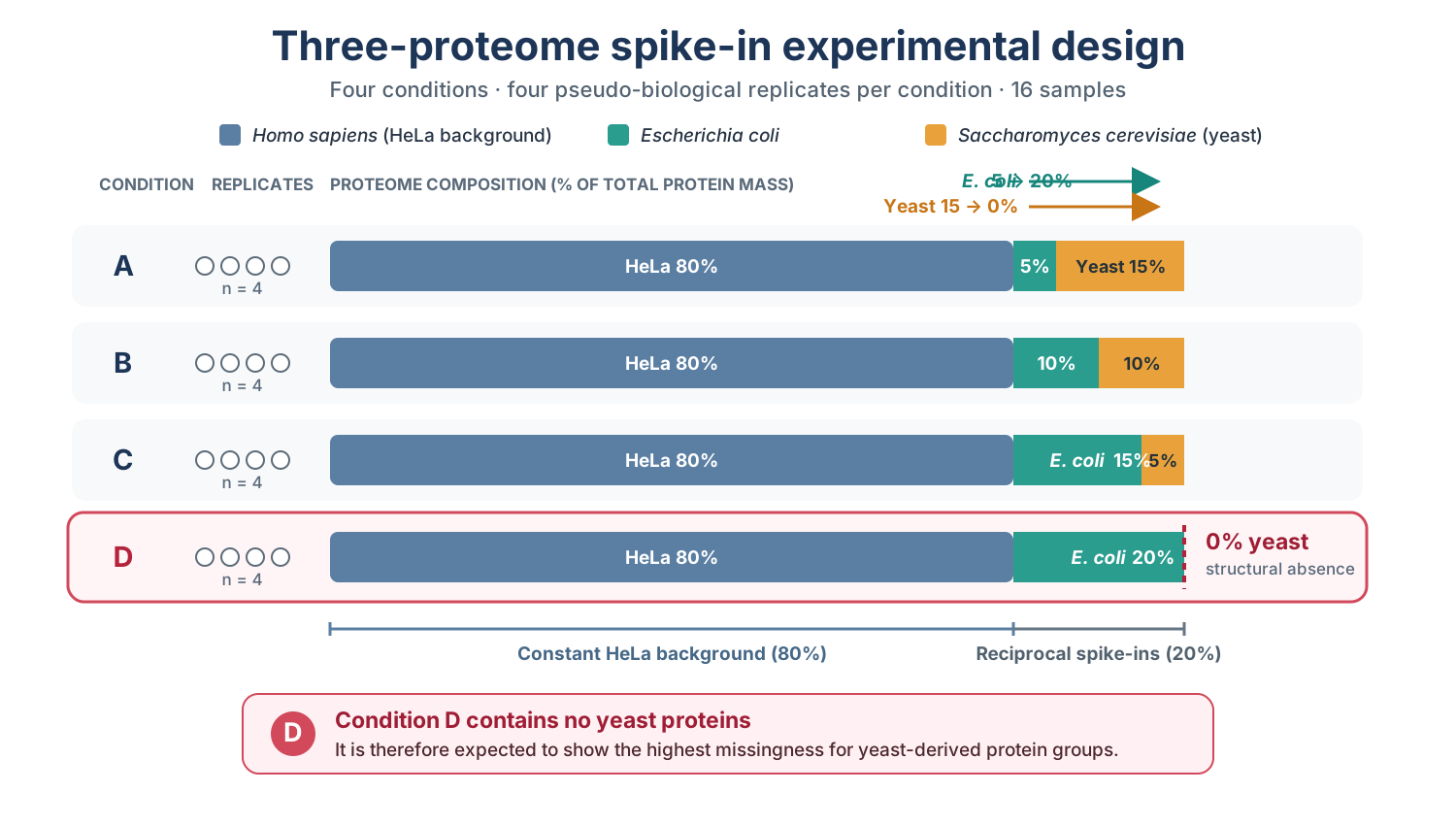
Complete three-proteome spike-in design underlying the example datasets. For distribution with NADIA, the datasets retain conditions A, B and D and 2,000 protein groups.

Click the figure to enlarge it; press Esc or click outside the image to close it.

Condition D contains no yeast proteins. This structural absence means that yeast-derived protein groups are expected to show the greatest proportion of missing values in D, making this condition particularly informative for demonstrating NADIA’s missing-value-aware filtering, imputation and differential abundance workflow.

To protect unpublished results from an ongoing study and comply with Bioconductor package-size constraints, the datasets distributed with NADIA are reduced to 2,000 protein groups and three representative conditions—A, B and D—with four replicates per condition. Condition D is deliberately retained because its absence of yeast proteins provides an informative biological missingness scenario.

The 2,000 protein groups were selected at random from the full report using a fixed seed, rather than by retaining the proteins with the highest abundance or the most complete measurements. This is important because selecting only the best-quantified proteins would remove much of the missingness that NADIA is designed to examine. Random selection retains a missing-value structure close to that of the full experiment, including condition-specific non-detection patterns. Because selection was also independent of measured intensity, it does not deliberately enrich the example for high-abundance proteins. The observed abundance distribution should therefore be regarded as a representative approximation of the full experiment, although it was not explicitly forced to match it through stratified sampling.

The reduced DIA dataset used in this vignette was derived from a Spectronaut quantification report and therefore contains 12 samples and 2,000 protein groups.

The dataset is available in two forms. The first is a compressed quantification report, which allows the import and preprocessing steps to be shown from the beginning:

report <- system.file("extdata", "nadia_dia_report.tsv.gz", package = "NADIA")
dia <- preprocess_spectronaut(report, condition_order = c("A", "B", "D"),
                              verbose = FALSE)
dia
#> Preprocessed Spectronaut data
#> -----------------------------
#> Runs (metadata): 12 
#> Proteins (ID): 2000 
#> Proteins (QUANT): 2000 
#> 
#> Conditions: A, B, D

preprocess_spectronaut() converts the long-format report—one row for each reported combination of run and protein group—into an object of class proteomics_data.

A proteomics_data object separates the information contained in the report into three coordinated tables:

• metadata contains one row per sample or LC-MS run, including the sample identifier, experimental condition, replicate, and any available run-level information;
• protein_id contains identification-level information for each protein group, including protein and gene annotations and, when available, run-specific evidence such as peptide and precursor counts, sequence coverage, and identification scores;
• protein_quant contains the protein-level quantification data. It includes the abundance measured for each protein group in each sample, together with the protein annotation and quantitative evidence required by the downstream workflow.

In this example, metadata contains 12 samples, whereas protein_id and protein_quant each contain 2,000 protein groups.

The three tables have different roles. metadata defines the experimental design, protein_quant provides the abundance matrix used for normalisation, imputation and differential abundance analysis, and protein_id retains the more detailed identification evidence for inspection and reporting.

Here, condition_order = c("A", "B", "D") selects the conditions to retain and sets the order used in the subsequent stages of the analysis.

The same dataset is also distributed as an already preprocessed object, allowing the remainder of the workflow to be run without reading the report again:

data(nadia_dia)
identical(dim(nadia_dia$protein_quant), dim(dia$protein_quant))
#> [1] TRUE

nadia_dia is the object used throughout the rest of this vignette.

How missing values are represented

Before processing the data, it is useful to check how missing values are represented because the encoding depends on the export format.

The Spectronaut report used here is in long format: each row corresponds to a reported combination of run and protein group. When no quantification is available for a particular combination, that combination is absent from the report. When preprocess_spectronaut() converts the report into the wide protein_quant matrix, it completes the grid of protein groups and samples and represents combinations absent from the report as NA:

quant <- as.matrix(nadia_dia$protein_quant[
    grep("^PG.Quantity_", colnames(nadia_dia$protein_quant))])

round(100 * mean(is.na(quant)), 1)          # percentage of missing intensities
#> [1] 8.1
round(100 * mean(rowSums(is.na(quant)) == 0), 1)  # complete proteins
#> [1] 72.2

In the full experiment from which this reduced dataset was obtained, 11,679 of the 16 × 10,437 possible combinations of samples and protein groups were absent, corresponding to approximately 7% of the matrix. In nadia_dia, around 8% of the intensities are missing and approximately one quarter of the protein groups contain at least one missing value.

These missing entries are subsequently handled according to the filtering and imputation settings selected for the analysis.

Other export formats may encode absence differently. An empty cell may be converted directly to NA during import, and NaN is also recognised as missing by functions such as is.na(). Some reports use zero as a marker of absence. In an intensity matrix, zero requires explicit treatment because log2(0) produces -Inf rather than a missing value.

For this reason, normalize_proteomics() converts values equal to zero into NA before applying the logarithmic transformation and reports the number of conversions when verbose = TRUE. No conversion is performed for nadia_dia because the example matrix contains no zeros.

At this stage, no assumption is made about whether an individual missing value should be regarded as MAR or MNAR. vignette("missing-values") describes the working assumptions used by NADIA and explains how missing values are assigned to the available imputation strategies.

Filtering, log2 transformation and normalisation

Before imputation and statistical analysis, NADIA prepares the quantitative matrix in three stages. First, values equal to zero are represented as NA, and proteins are retained according to their presence within the experimental groups. The filtering criteria are controlled by two arguments in process_proteomics():

• min_reps_filter is the minimum number of quantified replicates that a protein must have within a condition for that condition to satisfy the filter. When it is NULL, NADIA uses half the number of replicates in the smallest condition, rounded down. In nadia_dia, all conditions contain four replicates, so the automatically selected value is two;
• min_groups_filter is the minimum number of conditions that must satisfy min_reps_filter. Its default value is one, meaning that a protein is retained if it has sufficient observations in at least one condition.

The effect of the two criteria can be examined without running the later stages of the workflow. normalize_proteomics() exposes the same arguments as min_reps and min_groups, respectively. The following code applies several combinations and records how many of the 2,000 protein groups are retained or removed:

filter_grid <- expand.grid(
    min_reps_filter   = 1:4,
    min_groups_filter = 1:3
)

filter_counts <- do.call(rbind, lapply(seq_len(nrow(filter_grid)), function(i) {
    filtered <- normalize_proteomics(
        nadia_dia,
        min_reps    = filter_grid$min_reps_filter[i],
        min_groups  = filter_grid$min_groups_filter[i],
        norm_method = "log2",
        verbose     = FALSE
    )$filter_summary

    data.frame(
        min_reps_filter   = filter_grid$min_reps_filter[i],
        min_groups_filter = filter_grid$min_groups_filter[i],
        proteins_before   = filtered$n_total,
        proteins_retained = filtered$n_keep,
        proteins_filtered = filtered$n_drop
    )
}))

filter_counts
#>    min_reps_filter min_groups_filter proteins_before proteins_retained
#> 1                1                 1            2000              2000
#> 2                2                 1            2000              1997
#> 3                3                 1            2000              1986
#> 4                4                 1            2000              1962
#> 5                1                 2            2000              1997
#> 6                2                 2            2000              1984
#> 7                3                 2            2000              1953
#> 8                4                 2            2000              1877
#> 9                1                 3            2000              1712
#> 10               2                 3            2000              1607
#> 11               3                 3            2000              1533
#> 12               4                 3            2000              1444
#>    proteins_filtered
#> 1                  0
#> 2                  3
#> 3                 14
#> 4                 38
#> 5                  3
#> 6                 16
#> 7                 47
#> 8                123
#> 9                288
#> 10               393
#> 11               467
#> 12               556

The default filtering rule for this dataset corresponds to min_reps_filter = 2 and min_groups_filter = 1: it retains 1,997 of the 2,000 protein groups. Increasing either parameter makes the criterion more stringent. For example, requiring all four replicates in all three conditions retains 1,444 protein groups and removes 556.

Second, the retained intensities are transformed to the log2 scale. Third, NADIA applies the method selected through norm_method. Thirteen options are available, including log2, which retains the log2-transformed values without additional normalisation. The untransformed matrix (the raw assay), the log2-transformed matrix and the normalised matrix are kept as separate assays in the resulting SummarizedExperiment whenever they represent distinct processing stages.

The Normalisation section of vignette("choosing-methods") shows how to run and compare alternative normalisation methods. A separate optional filter, max_na_prop, can remove proteins with a high overall proportion of missing values immediately before imputation; it is disabled by default and is documented in ?impute_proteomics.

Imputation of missing values

Normalisation makes sample distributions more comparable, but it does not replace the values that remain missing. By default, NADIA therefore applies an imputation stage to the normalised matrix. Imputation estimates plausible values for missing entries from the observed data or from a model of the missingness mechanism. These estimates allow the subsequent analysis to use a complete matrix, but they are not new measurements and should not be interpreted as the unknown true values.

NADIA provides 20 selectable imputation strategies through imp_method. They include methods designed for MAR or MNAR values, the hybrid combo and softHybrid strategies, and none, which leaves missing values unchanged. The new halfmin option implements half-minimum imputation: each missing intensity is replaced with half the global observed minimum across all runs. The limpa route also avoids filling the missing entries and instead accounts for them in its probabilistic differential abundance model.

Each imputed result is stored as a new assay without overwriting the normalised matrix from which it was generated. vignette("missing-values") describes the assumptions behind all available methods, explains how combo and softHybrid assign missing values to different branches, and shows how the choice of strategy can affect the differential abundance results.

The workflow in a single call

process_proteomics() coordinates the main stages of the analysis: filtering, log2 transformation, normalisation, optional batch-effect correction, imputation of missing values, and differential abundance analysis. The function returns in memory the objects and tables required to inspect, visualise and export the results.

The concise syntax does not, however, represent a parameter-free analysis. Every omitted argument is assigned either a fixed default or a value resolved from the data or the selected method. Using the short call therefore means accepting the following principal analytical choices:

Stage	Default choice	Where it is explained
Filtering	min_reps_filter = NULL is resolved automatically (two replicates for this dataset), and min_groups_filter = 1 requires the criterion in at least one condition	Filtering, log2 transformation and normalisation above
Normalisation	cycloess, using the fast algorithm, three iterations and a span of 0.7	Filtering, log2 transformation and normalisation above and the Normalisation section of vignette("choosing-methods")
Batch correction	Not applied (batch_correct = FALSE)	vignette("batch-correction")
Imputation	combo, using Impseqrob for the MAR branch and min for the MNAR branch	Imputation of missing values above and vignette("missing-values")
Differential abundance	All pairwise comparisons with limma; alpha = 0.05 and no additional log2 fold-change threshold	Differential abundance results below
Covariates and blocking	No additional covariates, paired design or biological-replicate blocking	vignette("batch-correction")
File export	No files are written because export_dir = NULL; all results remain available in memory	vignette("results-and-export")

The complete call is shown below for transparency. Arguments that belong to an inactive branch, such as the batch-correction settings when batch_correct = FALSE, are still displayed so that the configuration can be inspected in full.

Show the complete call and all default arguments

res <- process_proteomics(
    preprocessing = nadia_dia,

    # File export
    export_dir = NULL,

    # Filtering
    min_reps_filter = NULL,
    min_groups_filter = 1,

    # Normalisation
    norm_method = "cycloess",
    cyclic_loess_method = "fast",
    cyclic_loess_iterations = 3,
    cyclic_loess_span = 0.7,

    # Optional batch correction
    batch_correct = FALSE,
    batch_column = "Batch",
    batch_algorithm = "ComBat",
    batch_ComBat_mode = 1,
    batch_covariates = NULL,
    batch_qualitycontrol = FALSE,

    # Imputation
    imp_method = "combo",
    mar_method = "Impseqrob",
    mnar_method = "min",
    prop_na_mnar = 0.51,
    prop_present_mar = 0.5,
    min_present_mar = 1,
    require_n_conditions = 1,
    max_na_prop = NULL,
    method_args = list(),
    with_value = NA_real_,

    # Differential abundance
    comparisons = NULL,
    control = NULL,
    logFC_threshold = 0,
    alpha = 0.05,
    eBayes_trend = NULL,
    eBayes_robust = NULL,
    de_method = "limma",

    # Covariates, paired designs and blocking
    covariate_df = NULL,
    covariate_column = NULL,
    bio_replicate_column = NULL,

    # Exported objects (used only when export_dir is supplied)
    export_normalized = TRUE,
    export_imputed = TRUE,
    export_format = "tsv",
    export_volcano = TRUE,
    export_boxplot = TRUE,
    export_pca = TRUE,

    # Progress messages
    verbose = TRUE
)

Accepting this configuration allows the complete analytical workflow to be reduced to a single line. In the executable call below, verbose = FALSE is used only to suppress progress messages in the vignette; its default is TRUE, and changing it does not affect the analysis.

res <- process_proteomics(nadia_dia, verbose = FALSE)
res
#> === Proteomics Processing Result ===
#> 
#> SummarizedExperiment:
#>   - Proteins: 1997 
#>   - Samples: 12 
#>   - Assays: raw, log2, cycloess, Impseqrob_min 
#>   - Conditions: A, B, D 
#> 
#> Differential Results:
#>   - Total rows: 5991 
#>   - Comparisons: B-A, D-A, D-B 
#>     B-A: Up=325, Down=172
#>     D-A: Up=374, Down=383
#>     D-B: Up=286, Down=382
#> 
#> Parameters:
#>   - Normalization: cycloess 
#>     - Cyclic Loess method: fast 
#>     - Cyclic Loess iterations: 3 
#>     - Cyclic Loess span: 0.7 
#>   - Imputation: combo 
#>     - MAR method: Impseqrob 
#>     - MNAR method: min 
#>   - Alpha: 0.05 
#>   - logFC threshold: 0 
#>   - Output directory: (no export)

For de_method = "limma", the unresolved eBayes_trend = NULL and eBayes_robust = NULL settings are both resolved to TRUE. Similarly, comparisons = NULL and control = NULL request all pairwise comparisons among the retained conditions.

These defaults provide a reasonable starting point, but they are not a universally optimal choice. vignette("choosing-methods") shows how to compare the alternatives on the data themselves, while vignette("missing-values") explains the assumptions underlying the available imputation strategies.

Where the processed data are stored

During processing, NADIA stores the quantitative matrices in a SummarizedExperiment, the standard Bioconductor container for matrix-like omics data. This object retains the input, log2-transformed and normalised matrices and, when the corresponding stages are applied, the batch-corrected and imputed matrices. Each matrix is stored as a separate assay, so the object contains both the intermediate processing stages and the normalised-and-imputed matrix used for downstream differential abundance analysis.

A SummarizedExperiment keeps three coordinated components:

• assays contain one or more quantitative matrices of identical shape, with protein groups in rows and samples in columns;
• rowData contains one row of annotation for each protein group;
• colData contains one row of metadata for each sample, including the experimental condition and replicate used to define the design.

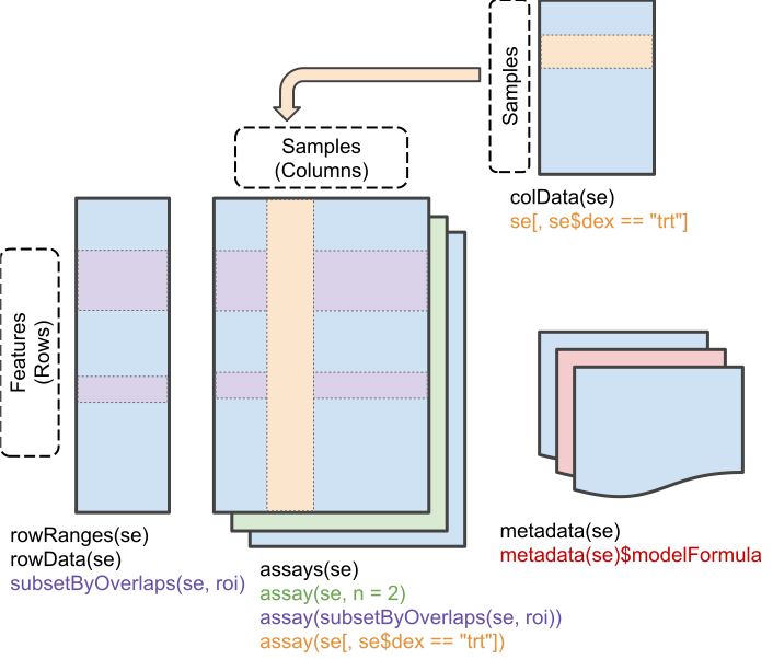
Structure of a SummarizedExperiment object.

Figure reproduced from the SummarizedExperiment source repository, distributed under the Artistic-2.0 licence.

These components share the same row and column indexing. Consequently, subsetting the object also subsets the corresponding protein annotation and sample metadata, preventing quantitative values from becoming misaligned with their identifiers or experimental groups.

During processing, the sample information required for the experimental design is stored in colData, the protein-group annotation required downstream is stored in rowData, and every quantitative stage is retained as a separate assay. The detailed protein_id table remains part of the original proteomics_data object and can be inspected separately when identification-level information is required.

The processed object is available as res$se_proc:

SummarizedExperiment::assayNames(res$se_proc)
#> [1] "raw"           "log2"          "cycloess"      "Impseqrob_min"

In this analysis, the assays correspond to successive stages of the workflow:

• raw, the input quantification matrix;
• log2, the matrix after log2 transformation;
• cycloess, the normalised matrix;
• Impseqrob_min, the matrix after the hybrid imputation.

The Impseqrob_min assay is the complete quantitative matrix obtained after the successive normalisation and imputation stages. In this analysis, it contains the intensities normalised with cycloess, with the remaining missing values filled by the default combo strategy: Impseqrob for values assigned to the MAR branch and min for values assigned to the MNAR branch. Thus, the data in Impseqrob_min are both normalised and imputed, and this is the matrix used as input for the subsequent differential abundance analysis. The assay name records the two imputation methods, although complete reproducibility also requires recording the normalisation method, the function arguments and the NADIA version.

Differential abundance results

res$DEPs_results holds the main table of the differential abundance analysis:

head(res$DEPs_results, 4)
#>         Protein.IDs Comparison Gene.Names       logFC     P.Value   adj.P.Val
#> 1        A0A024RBG1        B-A     NUDT4B  0.08293965 0.533563708 0.738922832
#> 2        A0A024RBG1        D-A     NUDT4B -0.01391145 0.916061045 0.951169322
#> 3        A0A024RBG1        D-B     NUDT4B -0.09685110 0.468736877 0.715101256
#> 4 A0A140T897;P02769        B-A        ALB  0.13439560 0.000573106 0.003118509
#>      Change         Assay MissGlobal MissComp MissCND1 MissCND2
#> 1 No Change Impseqrob_min          0        0        0        0
#> 2 No Change Impseqrob_min          0        0        0        0
#> 3 No Change Impseqrob_min          0        0        0        0
#> 4        Up Impseqrob_min          0        0        0        0

Each row corresponds to a combination of protein group and comparison. The same protein group may therefore appear in several rows if it takes part in more than one comparison.

The pairwise comparisons are built automatically from the conditions and the order defined during preprocessing:

res$comparisons
#> [1] B-A D-A D-B
#> Levels: B-A D-A D-B
table(res$DEPs_results$Change, res$DEPs_results$Comparison)
#>            
#>              B-A  D-A  D-B
#>   Up         325  374  286
#>   Down       172  383  382
#>   No Change 1500 1240 1329

The Change column classifies each result as Up, Down or No Change by applying the thresholds specified through alpha and logFC_threshold together:

• Up: adj.P.Val < alpha and a positive logFC, with logFC >= logFC_threshold;
• Down: adj.P.Val < alpha and a negative logFC, with logFC <= -logFC_threshold;
• No Change: does not satisfy both the adjusted-p-value and logFC criteria.

Here, alpha is the significance threshold applied to the adjusted p-value stored in adj.P.Val; it is not the adjusted p-value itself. With the default alpha = 0.05, a result must have adj.P.Val < 0.05 to be classified as significant. The unadjusted p-value remains available in P.Value, but it is not used to assign the default Change label.

The default logFC_threshold = 0 does not impose an additional minimum effect-size requirement. Consequently, a significant result with logFC > 0 is classified as Up, whereas one with logFC < 0 is classified as Down. Setting a positive threshold would require the logFC to be at least that value for Up or at most its negative value for Down.

Change is an interpretive label, not an additional statistical test. The underlying evidence remains in logFC, P.Value and adj.P.Val, and those values should be consulted whenever the magnitude and the uncertainty of a result need to be interpreted.

Relationship with the missing values

When imputation has been applied, the statistical result must be interpreted together with the information about the values that were missing before that stage.

NADIA keeps four columns, which go from the widest scope to the narrowest:

• MissGlobal, the percentage of missing values of the protein group across every sample in the experiment, including the conditions that take no part in the comparison. It therefore does not depend on the comparison: a given protein group carries the same value in all of them.
• MissComp, the percentage across the replicates of the two conditions being compared, and only those. This is the figure that describes the evidence actually available for that contrast.
• MissCND1 and MissCND2, the percentages in each of the two conditions separately. In a B-A comparison, MissCND1 corresponds to the numerator
  2. and MissCND2 to the denominator (A).

The distinction between the first two matters as soon as an experiment has more than two conditions, as this one does. MissGlobal is a property of the protein group in the experiment, so it does not move from one comparison to the next; MissComp does, because the replicates it counts change with the contrast. A protein group that is missing in a single replicate of D shows both behaviours at once:

pid <- with(res$DEPs_results, Protein.IDs[MissGlobal != MissComp][1])
subset(res$DEPs_results, Protein.IDs == pid,
       c("Comparison", "MissGlobal", "MissComp", "MissCND1", "MissCND2"))
#>    Comparison MissGlobal MissComp MissCND1 MissCND2
#> 46        D-A       8.33     12.5       25        0
#> 47        B-A       8.33      0.0        0        0
#> 48        D-B       8.33     12.5       25        0

MissGlobal describes how well the protein group is covered in the experiment as a whole, which is useful for deciding how much to trust it at all. MissComp and the two per-condition columns describe the support behind one particular contrast. None of them determines whether a change is biologically real, but together they distinguish estimates based mainly on measured intensities from estimates that depend largely on imputed values.

The relationship between missingness and the differential call can be summarised directly. MissComp is the right column here, because what is being related to the call is the evidence available for that particular contrast:

bins <- cut(res$DEPs_results$MissComp, c(-1, 0, 25, 50, 100),
            labels = c("0%", "1-25%", "26-50%", ">50%"))
table(missing = bins, res$DEPs_results$Change)
#>         
#> missing    Up Down No Change
#>   0%      795  209      3761
#>   1-25%    90   57       239
#>   26-50%   70  619        54
#>   >50%     30   52        15

In this example dataset, most results with no missing values are called No Change. Among results with 26–50 % missing values, by contrast, there is a marked asymmetry: 619 are called Down against 70 called Up.

This pattern does not prove that all those missing values are MNAR, but it is consistent with a substantial abundance-dependent component of missingness. When a protein group stops being quantified in one condition, values imputed from the lower end of the distribution can produce a large negative change.

Interpretation must always be made in the context of the missingness pattern and the imputation method used.

Detection and non-detection patterns between conditions

The most extreme case occurs when a protein group is not quantified in any replicate of one condition but is quantified in every replicate of the other:

onoff <- subset(res$DEPs_results,
                (MissCND1 == 100 & MissCND2 == 0) |
                (MissCND1 == 0   & MissCND2 == 100))
nrow(onoff)
#> [1] 500
head(onoff[, c("Protein.IDs", "Comparison", "logFC", "adj.P.Val",
               "MissCND1", "MissCND2")], 4)
#>     Protein.IDs Comparison      logFC    adj.P.Val MissCND1 MissCND2
#> 157      O13535        D-A -11.097985 5.054321e-18      100        0
#> 158      O13535        D-B -10.603939 8.186147e-18      100        0
#> 161      O13563        D-A  -8.281384 1.823333e-16      100        0
#> 162      O13563        D-B  -7.689337 3.907152e-16      100        0

Roughly 500 results in this analysis have 100 % missing values in one group and 0 % in the other. These are detection versus non-detection patterns between conditions. They may represent biologically relevant changes, but they require a different interpretation from a ratio calculated entirely from observed intensities.

A logFC of around −11, for example, should not be interpreted as a directly measured abundance ratio. Its magnitude depends largely on the value introduced by the MNAR method, and it states that one condition lies below the quantifiable range relative to the other.

The MissCND1 and MissCND2 columns make this distinction visible. In contrast, the p-value alone says nothing about how many observations were measured and how many were imputed. vignette("missing-values") develops this distinction and explains how the different imputation strategies affect these results.

Visualising the results

process_proteomics() prepares three tables that can be used directly by the visualisation modules:

• res$DEPs_results, for the volcano plots;
• res$BoxPlot_Input, to compare the sample distributions across the different assays;
• res$PCA_Input, for PCA and heatmaps.

The visualisation functions take these tables rather than the complete SummarizedExperiment, which means they can also be applied to results that have been modified or produced by other workflows, provided they keep the expected structure.

Interactive figures

NADIA produces interactive volcano plots, boxplots and PCA projections through Highcharts. Each function returns a named list whose elements correspond — depending on the module — to comparisons, assays or protein selection modes:

volcano <- volcano_highchart_list(res$DEPs_results)
boxplot <- boxplot_highchart_list(res$BoxPlot_Input)
pca     <- pca_highchart_list(res$PCA_Input)

volcano[["B-A"]]

volcano[["B-A"]], for example, selects the volcano plot for the B-A comparison.

The following static image provides a preview of that interactive volcano plot for the B-A comparison. It shows the results obtained from the matrix normalised with cycloess and imputed with the default Impseqrob_min strategy:

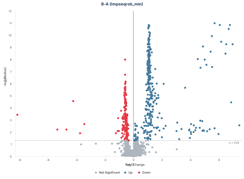
Static SVG preview of the interactive volcano plot for the B-A comparison using the cycloess-normalised and Impseqrob_min-imputed matrix.

Click the figure to enlarge it; press Esc or click outside the image to close it.

The interactive figures themselves are not rendered in this vignette, to keep the document small. vignette("visualization") shows interactive versions of the three modules and explains their main customisation options. vignette("results-and-export") describes how to save each widget as an HTML file.

All three take their input from res, so they can equally be built from a saved analysis: write_nadia() puts the whole thing — tables, parameters and provenance — into one file, and nadia_result() gives back an object these functions accept unchanged. See vignette("results-and-export").

Static figure

proteomics_heatmap() generates a static heatmap from res$PCA_Input and can also select which protein groups to display.

In the following example, mode = "target" restricts the figure to protein groups that are significant in the comparison specified by comparison:

hm <- proteomics_heatmap(
    res$PCA_Input,
    mode            = "target",
    comparison      = "B-A",
    scale_data      = "row",
    sample_order    = "condition",
    condition_order = c("A", "B", "D"),
    show_row_names  = FALSE,
    heatmap_title   = "Significant in B-A")
hm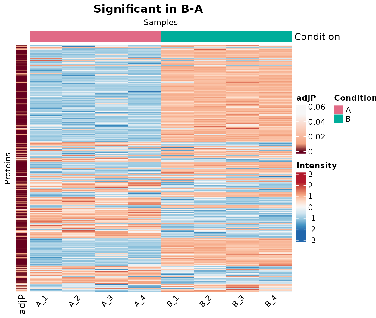

The figure uses the following options:

• comparison = "B-A" selects the comparison of interest;
• scale_data = "row" standardises the profile of each protein group separately, so that colour represents relative changes between samples rather than differences in absolute abundance between proteins;
• sample_order = "condition" groups the samples by condition;
• condition_order = c("A", "B", "D") sets the order of those conditions explicitly;
• show_row_names = FALSE hides the identifiers, which would otherwise be illegible when many rows are drawn.

The heatmap therefore shows the relative patterns of the selected protein groups across the A, B and D samples. It should not be interpreted as a map of absolute protein abundances.

Further options for selection, clustering, ordering and customisation are described in vignette("visualization").

Next steps

This vignette has shown the complete workflow using NADIA’s default configuration. Those defaults provide a reproducible starting point, but they should not be interpreted as the best choice for every dataset.

One of the decisions with the greatest effect on the final results table is the choice of normalisation and imputation methods. vignette("missing-values") explains the assumptions underlying the available strategies, whereas vignette("choosing-methods") shows how to compare them when no known reference is available. When the experiment contains a spike-in, vignette("benchmarking") evaluates them against the expected changes.

To import your own data, adjust figures or export the results, see the vignettes linked in the introduction.

Session information

sessionInfo()
#> R version 4.6.1 (2026-06-24)
#> Platform: x86_64-pc-linux-gnu
#> Running under: Ubuntu 24.04.4 LTS
#> 
#> Matrix products: default
#> BLAS:   /usr/lib/x86_64-linux-gnu/openblas-pthread/libblas.so.3 
#> LAPACK: /usr/lib/x86_64-linux-gnu/openblas-pthread/libopenblasp-r0.3.26.so;  LAPACK version 3.12.0
#> 
#> locale:
#>  [1] LC_CTYPE=C.UTF-8       LC_NUMERIC=C           LC_TIME=C.UTF-8       
#>  [4] LC_COLLATE=C.UTF-8     LC_MONETARY=C.UTF-8    LC_MESSAGES=C.UTF-8   
#>  [7] LC_PAPER=C.UTF-8       LC_NAME=C              LC_ADDRESS=C          
#> [10] LC_TELEPHONE=C         LC_MEASUREMENT=C.UTF-8 LC_IDENTIFICATION=C   
#> 
#> time zone: UTC
#> tzcode source: system (glibc)
#> 
#> attached base packages:
#> [1] stats     graphics  grDevices utils     datasets  methods   base     
#> 
#> other attached packages:
#> [1] NADIA_0.99.1     BiocStyle_2.40.0
#> 
#> loaded via a namespace (and not attached):
#>   [1] gridExtra_2.3.1             rlang_1.3.0                
#>   [3] magrittr_2.0.5              clue_0.3-68                
#>   [5] GetoptLong_1.1.1            otel_0.2.0                 
#>   [7] matrixStats_1.5.0           compiler_4.6.1             
#>   [9] png_0.1-9                   systemfonts_1.3.2          
#>  [11] vctrs_0.7.3                 stringr_1.6.0              
#>  [13] pkgconfig_2.0.3             shape_1.4.6.1              
#>  [15] crayon_1.5.3                fastmap_1.2.0              
#>  [17] backports_1.5.1             XVector_0.52.0             
#>  [19] rmarkdown_2.32              ragg_1.5.2                 
#>  [21] highcharter_0.9.5           purrr_1.2.2                
#>  [23] xfun_0.60                   cachem_1.1.0               
#>  [25] tidyHeatmap_1.13.1          jsonlite_2.0.0             
#>  [27] DelayedArray_0.38.2         broom_1.0.13               
#>  [29] parallel_4.6.1              cluster_2.1.8.2            
#>  [31] R6_2.6.1                    bslib_0.12.0               
#>  [33] stringi_1.8.9               RColorBrewer_1.1-3         
#>  [35] limma_3.68.5                rlist_0.4.6.2              
#>  [37] rrcov_1.7-7                 GenomicRanges_1.64.0       
#>  [39] lubridate_1.9.5             jquerylib_0.1.4            
#>  [41] Seqinfo_1.2.0               bookdown_0.48              
#>  [43] assertthat_0.2.1            SummarizedExperiment_1.42.0
#>  [45] iterators_1.0.14            knitr_1.51                 
#>  [47] zoo_1.9-0                   IRanges_2.46.0             
#>  [49] Matrix_1.7-5                splines_4.6.1              
#>  [51] timechange_0.4.0            tidyselect_1.2.1           
#>  [53] viridis_0.6.5               abind_1.4-8                
#>  [55] yaml_2.3.12                 doParallel_1.0.17          
#>  [57] codetools_0.2-20            curl_8.0.0                 
#>  [59] lattice_0.22-9              tibble_3.3.1               
#>  [61] S7_0.2.2                    Biobase_2.72.0             
#>  [63] quantmod_0.4.29             withr_3.0.3                
#>  [65] evaluate_1.0.5              desc_1.4.3                 
#>  [67] rrcovNA_0.5-3               xts_0.14.2                 
#>  [69] norm_1.0-11.1               circlize_0.4.18            
#>  [71] pillar_1.11.1               BiocManager_1.30.27        
#>  [73] MatrixGenerics_1.24.0       foreach_1.5.2              
#>  [75] stats4_4.6.1                pcaPP_2.0-5                
#>  [77] generics_0.1.4              TTR_0.24.4                 
#>  [79] ggplot2_4.0.3               S4Vectors_0.50.2           
#>  [81] scales_1.4.0                glue_1.8.1                 
#>  [83] tools_4.6.1                 dendextend_1.19.1          
#>  [85] robustbase_0.99-7           data.table_1.18.6.1        
#>  [87] reactable_0.4.5             fs_2.1.0                   
#>  [89] mvtnorm_1.4-2               grid_4.6.1                 
#>  [91] tidyr_1.3.2                 colorspace_2.1-3           
#>  [93] patchwork_1.3.2             cli_3.6.6                  
#>  [95] textshaping_1.0.5           viridisLite_0.4.3          
#>  [97] S4Arrays_1.12.0             ComplexHeatmap_2.28.0      
#>  [99] dplyr_1.2.1                 gtable_0.3.6               
#> [101] DEoptimR_1.2-1              sass_0.4.10                
#> [103] digest_0.6.39               BiocGenerics_0.58.1        
#> [105] SparseArray_1.12.2          farver_2.1.2               
#> [107] rjson_0.2.23                htmlwidgets_1.6.4          
#> [109] htmltools_0.5.9             pkgdown_2.2.1              
#> [111] lifecycle_1.0.5             GlobalOptions_0.1.4        
#> [113] statmod_1.5.2